Replication of Rosgen Stream Classification Analysis

Background

This analysis is a replication of two analyses. The original, performed by David Rosgen, took information from studies of multiple river systems to devise a classification scheme based on a number of factors, including the width of the valley and of the river when full, slope, and even particle size of material (e.g. pebbles, sand) on the riverbed. The second was a study conducted by Alan Kasprak, et. al., which applied Rosgen’s framework to Oregon’s John Day River.

In conducting this analysis, students like myself were assigned points from Kasprak’s study at random to study. Through open source GIS and analytical tools like R/RStudio and GRASS GIS, we attempted to use data from the Columbia Habitat Monitoring Program - a project aiming to generate a standard set of fish habitat monitoring methods in and around the Columbia River, LIDAR DEMs at 1m resolution, and models developed from these data to gather sufficient data for analysis.

Sampling Plan and Data Description

As stated earlier, each student conducting this analysis was assigned a data point from Kasprak’s analysis in the CHaMPs data. My designated location was at loc_id=4, and two sampled points existed, from which I chose at random.

Materials and Procedure

In performing this analysis, we followed workflows pre-prepared by ASU Geography PhD candidate Zach Hilgendorf in collaboration with Middlebury College assistant professor Joseph Holler, working in both GRASS GIS and RStudio. The workflow followed in grass is linked here, the code run in RStudio is linked here, and the instructions for running the code in RStudio and eventually classify the stream at the assigned point are provided here.

Unfortunately, in working with Prof. Holler and other students enrolled in this course, we discovered that we were unable to properly unzip the DEM data, requiring the use of a tool like Unarchiver, and issues arose installing tools within RStudio, requiring the installation of XCode within Apples developer tools.

Some tools created by Prof. Holler used in this analysis are included here:

• Centerlines tool
  • note: due to strange geography of the river at the assigned study site, a center line tool that does not clip is used here, requiring extra attention to ensure comparable lengths for the valley and stream centerlines. An additional tool that does clip can be found here

Replication Results

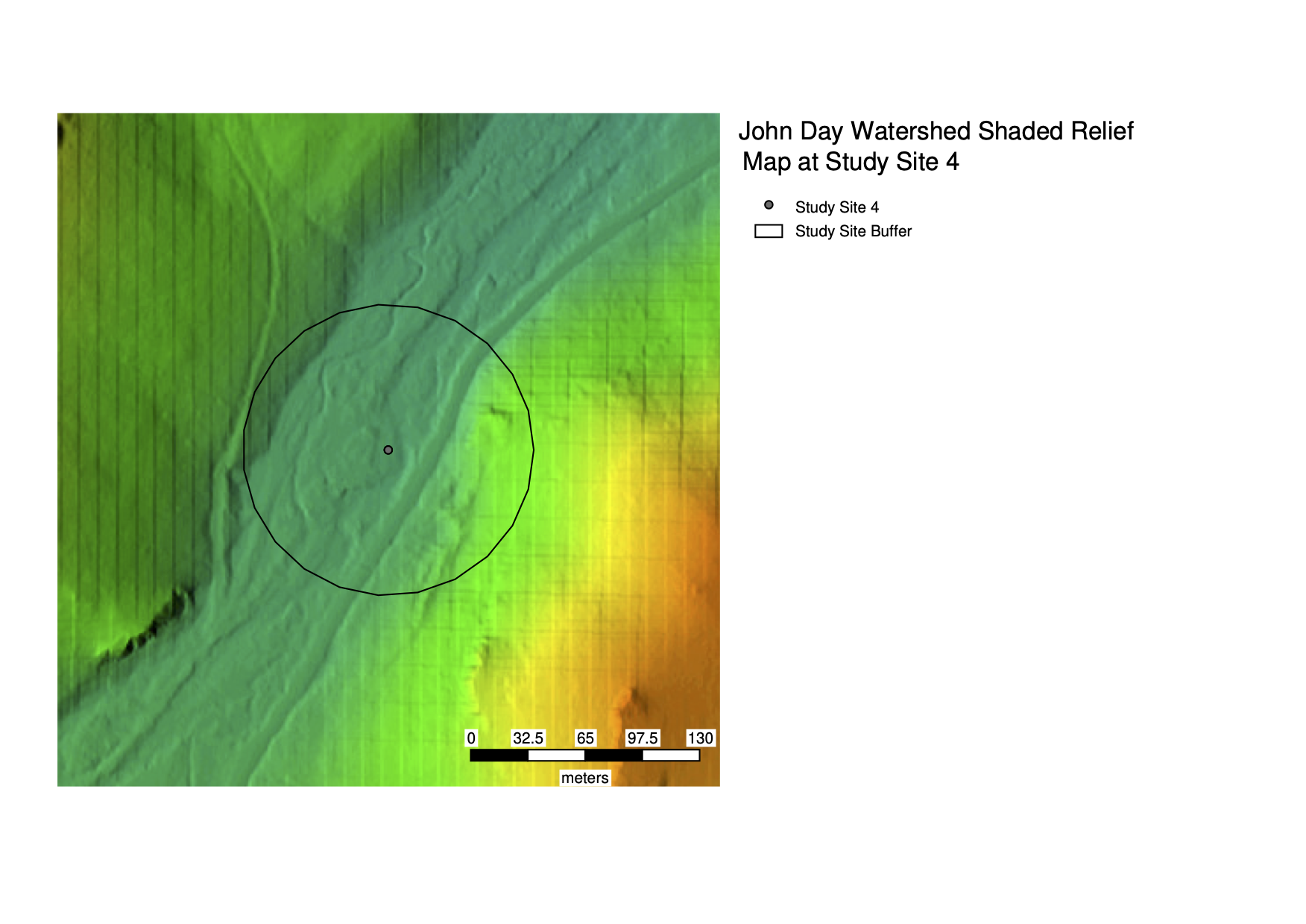
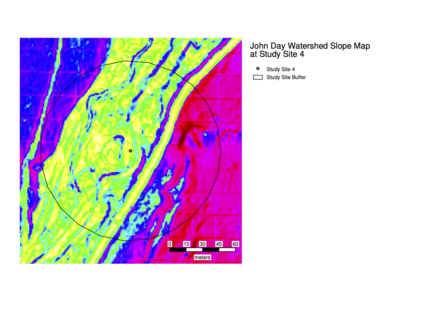
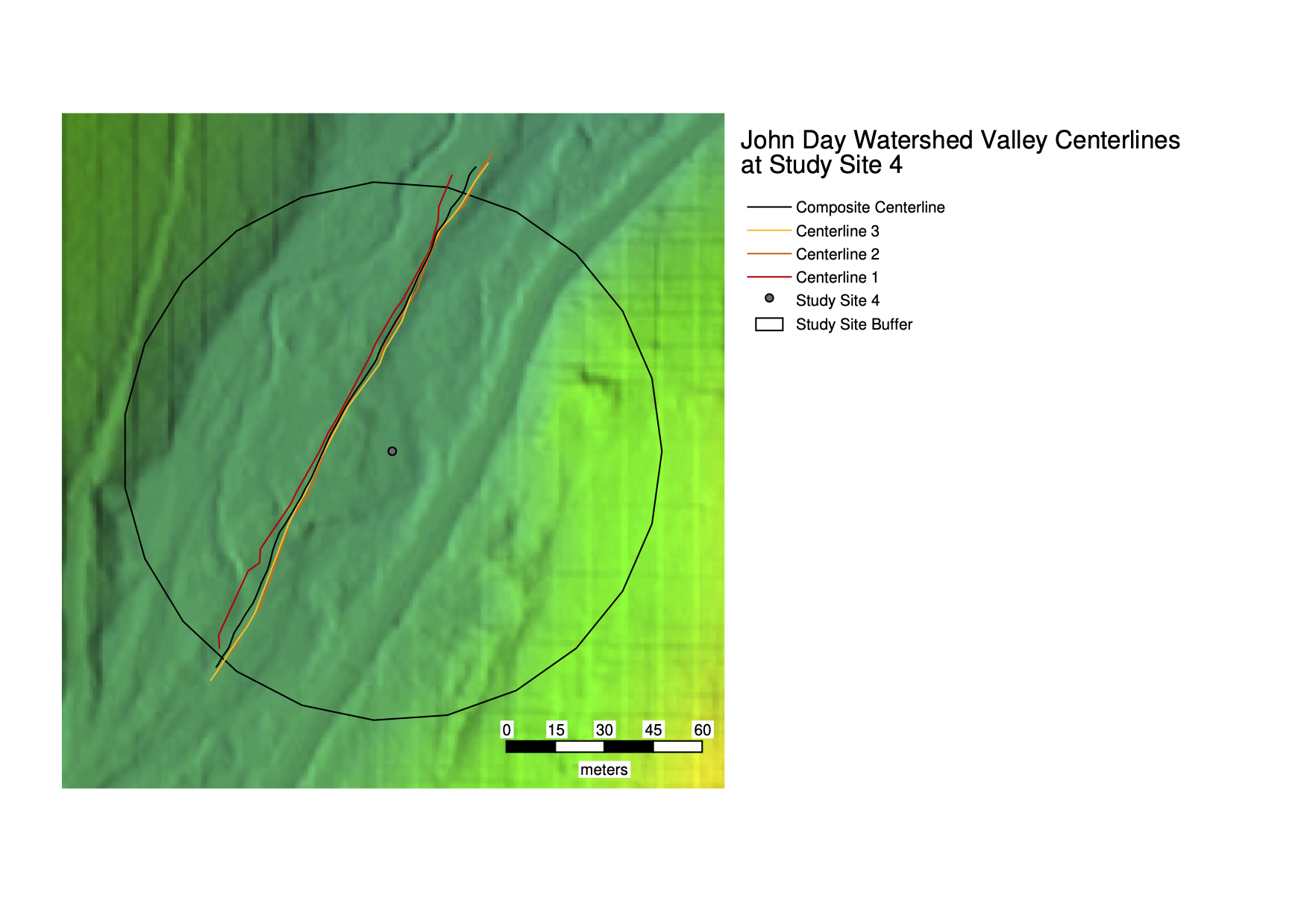
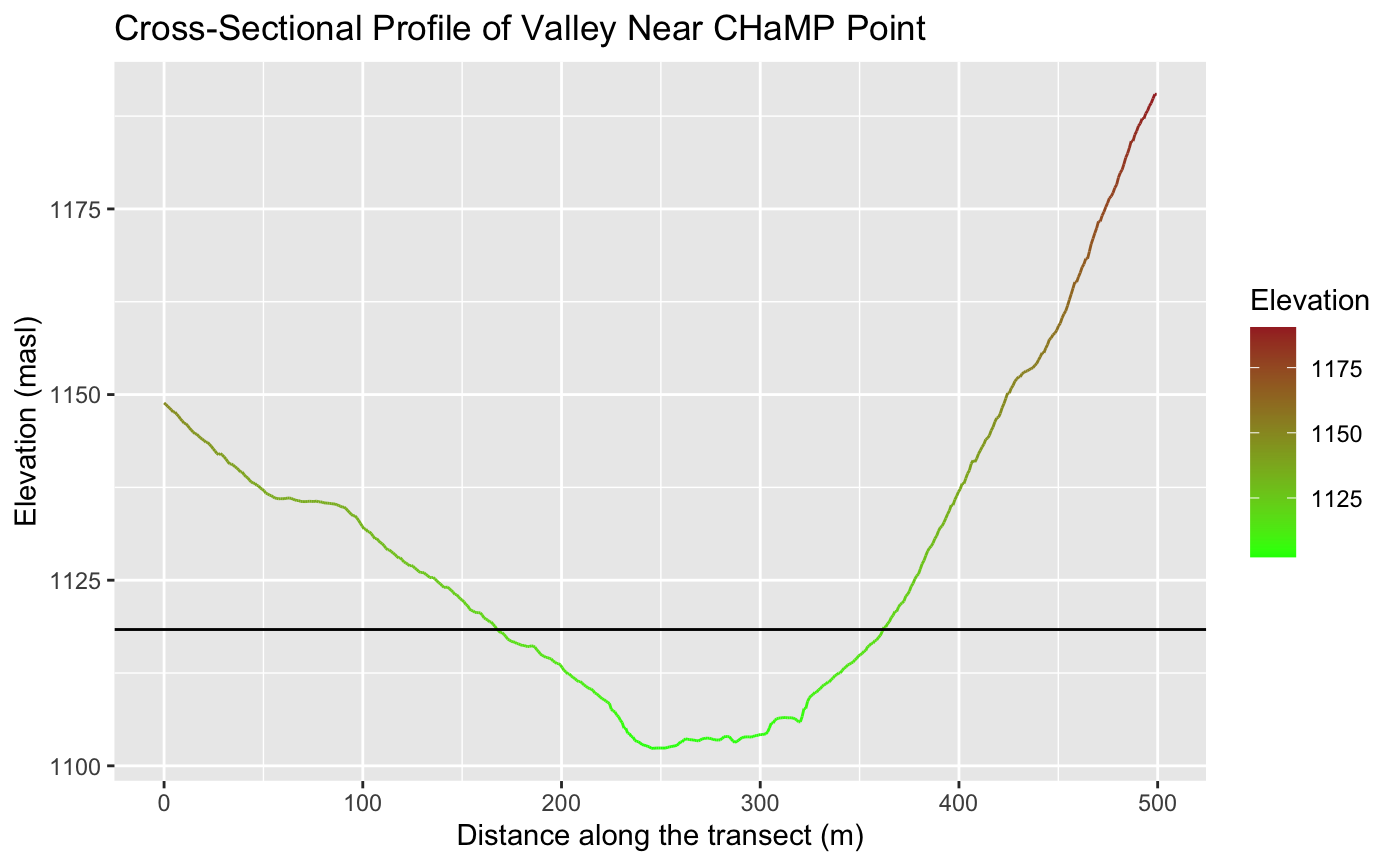
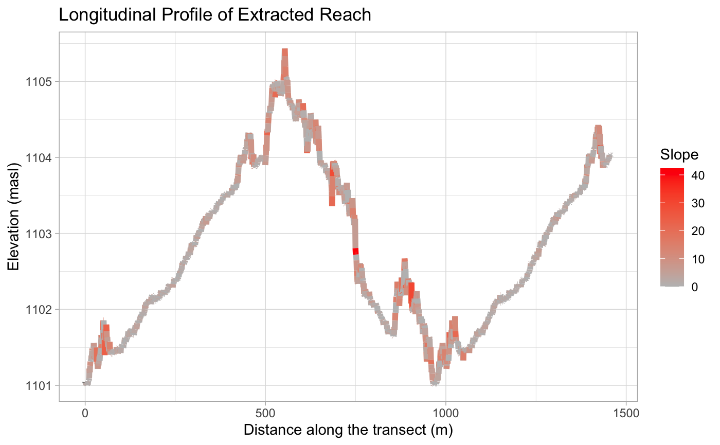
Table 1 Site Measurements

Variable	Value	Source
Bankfull Width	8.2643	BfWdth_Avg in CHaMP_Data_MFJD
Bankfull Depth Average	0.2732	DepthBf_Avg in CHaMP_Data_MFJD
Bankfull Depth Max	0.872	DepthBf_Max in CHaMP_Data_MFJD
Valley Width	60	Cross section profile
Valley Depth	1.744	2x bankfull depth max
Stream/River Length	184.4277	Grass measurement of bank centerline
Valley Length	174.0437	Grass measurement of valley centerline
Median Channel Material Particle Diameter	108	CHaMP

Table 2 Rosgen Level I Classification

Criteria	Value	Derivation
Entrenchment Ratio	7.260	valley width / bankfull width from Table 1
Width/Depth Ratio	30.25	bankfull width / bankfull average depth from Table 1
Sinuosity	1.059	stream length/valley length from Table 1
Level I Stream Type	C	The Key to the Rosgen Classification of Natural Rivers (Rosgen, 1994)

Table 3 Rosgen Level II Classification

Criteria	Value	Derivation
Slope	3.918474	ΔElevation/ΔDistance in the Longitudinal Profile
Channel Material	Cobbles	The Key to the Rosgen Classification of Natural Rivers (Rosgen, 1994)
Level II Stream Type	Unclear	The Key to the Rosgen Classification of Natural Rivers (Rosgen, 1994)

Discussion and Deviations from Protocol

Unfortunately, this stream has proven difficult to classify beyond Level I, with even that level containing some unforeseen difficulties. As seen in the longitudinal profile of the river, the elevation seems to go up and down repeatedly over the stream’s course, something which should not happen. Paired with the slope and elevation maps, this seems to indicate that this river may be comprised of multiple channels, and that the stream centerline may inadvertently be crossing the “banks” between these smaller stream channels; this throws off the measurement of the slope.

Looking at Rosgen’s classification schemes, the slope provided is unusable in any classification scheme. Ignoring that measurement and continuing on with stream type C as identified in table 2 - which may itself be in error, as the sinuosity does not quite match up with the other ratios, potentially an effect of a stream with multiple channels - then we can identify the stream as type C3, C3b, or C3c. The measured sinuosity fits with those corresponding to multi-channel streams, but following this classification further, the width/depth ratio found in this analysis does not allow us - under Rosgen’s scheme at least - to consider a stream with cobble as the primary channel material.

Conclusions

Ultimately, this analysis has not been entirely successful, with the classification scheme seeming to collapse under the information given in the CHaMPs data, and thus not successfully replicating the results of Kasprak et al (2016). GIS is an incredibly powerful tool that can detect a surprising amount of information, and when paired with data volunteered by scientists and community members - a la OpenStreetMap - is capable of wide reaching, widely varied analyses. Unfortunately, however, this replication seems to back up the idea that GIS is not limitless, and on the ground experience is just as valuable as geospatial analyses, especially considering the inconsistencies and uncertainties discussed here. While the classification of rivers from behind a computer screen represents an exciting innovation that could be deployed to understudied areas, an ongoing role of scientists and field work seems to be necessary, at least as a stopgap to help to clear up uncertainties when they arise.

Main Page

This work is licensed under a Creative Commons Attribution-NonCommercial-ShareAlike 4.0 International License.